Online Beam Natural Frequency Calculator

This active web form can be used to calculate the first 2 modes of a general beam configuration.  Up to 24 different beam segments can be used with each having different section and area properties including weight density.  Concentrated weights can also be added.  Boundaries include free, simple support and fixed slope.  Both vertical and rotational springs can also be used.

Output includes the first 2 mode frequencies in Hz and the respective mode shapes.  A gravitational constant must be defined.  All dimensional units must be consistent with each other and Hz.

A uniform beam of length = 24 inches, E = 30,000,000 psi, I = .25 in⁴, A = .28167 in², weight density of 0.3 lb/in³ gave the following results compared to theoretical values:

Cantilevered:
Model f₁ = 179.8; f₂ = 1124.4 versus theory of f₁ = 179.9; f₂ = 1127.5 Hz

Fixed End/Simple Supported End:
Model f₁ = 789.0; f₂ = 2556.9 versus theory of f₁ = 789.0; f₂ = 2556.7 Hz

Fixed End/Fixed End:
Model f₁ = 1144.9; f₂ = 3159.7 versus theory of f₁ = 1144.9; f₂ = 3155.8 Hz

Reference: Theory of Vibration with Applications, W. T. Thomson, 4th Edition.

Simply change or add values to any of the white cells and the frequencies are automatically updated.




The following screenshot is a more complex configuration and with all of the features used.

Complex Beam Configuration.

Expanded Web Beam Calculator

This is an expanded Beam Analysis version from an earlier posting.  This version has up to 24 segments available each with its own section properties and elastic modulus.  Available loads include concentrated vertical and moments.  Vertical and rotational springs are also available.  Boundary conditions include simple, slope and fixed.  Each can be "0" or specific values can be used.  Charts of results include displacement, moment, shear and top and bottom fiber stresses.  Maximum and minimum stresses and deflections are listed.

The following embedded Excel form is live.  Any "white" cell can be changed and the results are updated immediately.

Beam Designer

Updated: 3/14/2014 at 12:22 EST.  We found that some of the worksheet tabs had the entire sheet protection activated which made the entire sheet non-editable.  An undated version with all the tabs editable is available from the same link given below.  Apologies for any inconvenience.

The attached Excel spreadsheet is an extension of previously posted beam calculators on this blog and XL4Sim.  This one has two significant improved differences:

Beam Designer Dashboard.

1.  Rather than using the VBA module to do the beam calculations they are done directly via worksheet formulas.  This enables "instant" updates as changes are made to the input cells.  This makes scenario projects very fast. The cell formulas are on the same worksheet as the input cell sheet and, therefore, the sheet can be copied as many times as needed without loss of functionality.  Multiple workbooks can also be made.

2.  A VBA macro option is available on the worksheet that will "optimize" the beam configuration given a user list of available beam sections defined by area moment area of inertia and corresponding section moduli (top and bottom). The optimizer will find the combination of given beam sections optimized to the user defined maximum stress using the smallest sections. The ideal optimum is where all the beam segments are at the maximum allowable stress which will usually correspond to the lowest weight and many times the lowest cost.  The algorithm will consider the sections given by the user and will not become trapped in a local minimum.

It takes ~ 1-2 minutes to complete if the largest number of beam segments (24) and user input sections (21) are used.

Up to 24 beam segments can be used with each having different section properties.  For the optimizer the user can input up to 21 different sections to be considered.  The only restrictions are: 1) they be input from smallest area moment of inertia to largest and 2) the largest section, if used for the entire beam, will result in the maximum stress <= the target stress.  The program will provide caution messages for each condition.  In some cases the program will find sections that can be smaller than the ones the user has provided.  These will show up as being stressed less than the allowable.  The worksheet charts update after each cycle so you can watch as the optimization proceeds.

Available boundary conditions include simple-support with a given displacement value, fixed slope with a given value, and fixed displacement/slope.  Translational and rotational springs are also available.  Loads include concentrated forces and moments.  Moment, shear, stress and deflection charts are given.  The calculations are dimension neutral but they must be consistent.

As an aside,  the built-in Excel Solver optimizer can be used but it is not very practical for this type of application because it gets too easily trapped in local minimums and can not easily handle discrete changes to the variables.  The algorithm used in this spreadsheet is a guided descent approach which takes advantage of the known properties of the domain.

The spreadsheet download has several examples of trial cases (one per worksheet) that can be used as examples.  The VBA module and cell formulas in Range A150:DC700 are password protected to protect them from being broken or inadvertently overwritten.  The VBA module has been 3rd party code signed (Thawte) to help with the Excel security settings.  The VBA module is also date limited for 6 months.  See this blog or www.xl4sim.com for future updates.

Here are two examples.  The first, is a fix-ended beam with a center load but the section moduli of the bottom fiber is 1/2 the upper fiber.  The second is a bit more complex with an end moment, two vertical loads, a vertical spring, a fixed end and mid-span simple support. Note for each the optimizer tries to find a combination where each beam segment is close to the allowable stress which in these cases is 24ksi.  They won't quite reach the allowable stress because of the discrete sections.

Another potentially valuable feature is once the "optimum" is found the user can manually change any of the beam parameters and get an "instant" result for additional "what ifs".

Fix-Ended Beam with Center Load Example.

Complex Beam Example.

Online Euler Buckling Solver for Multiple Segment Axial Members

The subject online axial Euler buckling solver can determine the Euler buckling load for an axial member with up to 5 segments each with its own elastic modulus and area moment of inertia.  Boundary conditions of free, simple support, fixed slope and or elastic spring can be applied at the start and end of each segment.  The output includes the buckling load, maximum compression stress using the smallest input area and a slenderness ratio using the full length and smallest EA value.  The later two output parameters can be used to determine if Euler buckling is an adequate representation of the simulation.  Compression stress values approaching the material yield and low slenderness ratios suggest nonlinear buckling maybe more appropriate.

The calculator matches the classic Euler buckling equation P_cr = EI(π/KL)² for simple-simple (K=1), fixed-fixed (K=0.5), simple-fixed (K=0.7) and fixed-free (K=2) end conditions.




An extended version of this calculator which also includes a nonlinear option can be found at www.xl4sim.com.

Web Page Embedded Euler Beam Calculator

The Euler Beam Calculator shown below is a web page (this page) embedded active Excel spreadsheet.  It uses the Microsoft SkyDrive file sharing system and does not require the user to have Excel to use.

This calculator will solve a user defined multi-span beam.  Up to 5 beam segments can be input each with its own elastic modulus, bending area moment-of-inertia, and top and bottom section moduli. Concentrated loads and moments can be input along with slope and displacement boundary conditions.

The solution provides a deflection chart, moment and shear diagrams and stress plots.  The calculator updates immediately as cells are changed.

This calculator is active.  Change a cell and watch it update the solution.

Rubber State-of-Cure vs Time and Position

Rubber state of cure generally depends on the temperature time history during the mold cycle.  It can be a complex thermal kinetics problem due to the transient nature of the cure and temperature in time and position.  The attached MS Excel Macro is a temperature and state-of-cure calculator that has 5 molding configurations:  1) planar with one heated side; 2) planar with two heated sides; 3) cylindrical with a heated inner surface; 4) heated outer surface and 5) both inner and outer surfaces heated.  For these configurations it is assumed that the molded shape has a high length-to-thickness ratio allowing the problem to be treated 2-dimensionally.

The dashboard looks like this with a worksheet tab for each configuration.

Rubber State-of-Cure Calculator Dashboard.

The calculator uses the user input cure curve information for the rubber and the calculator solves the time/position/temperatures and the resulting state-of-cure versus time and position.

This section was added on 2/22/2014:

The implicit finite difference formulation is used to solve the for the temperatures in time and position. The implicit method is unconditionally stable in time, although this does not preclude using a small time step for improved accuracy.  Progressively decreasing the time step until convergence is always good practice.  The same is true for the spatial size. In this case the number of nodes.  Any number of good references are available that describe the methodology including Fundamentals of Heat and Mass Transfer by Incropera and DeWitt, 4th Edition.

This module assumes that the thermal properties (conductivity and specific heat) do not change over the temperature range and state-of-cure.  It also assumes there is no significant additional heating from the curing kinetics.

The MS Excel Macro has been code signed with a 3rd party code signing certificate to allow higher macro security settings.

A version enabling a larger range of shapes is underway.

Heat Sink Transient Response Benefits

Many thermal management systems have unsteady heat loads.  Heat sink design and/or selection can be considered with these unsteady loads in mind.

An example of a natural convection finned heat sink is used to show how the thermal mass of the heat sink can be used to reduce its required cooling capacity.  Generally the effects of thermal mass are intuitive but calculating the benefits can sometimes be challenging.  This example shows an easy and quick simulation for evaluating the potential benefits of the transient behavior.

XL4Sim Simulation of a Transient, Naturally Cooled Heat Sink.

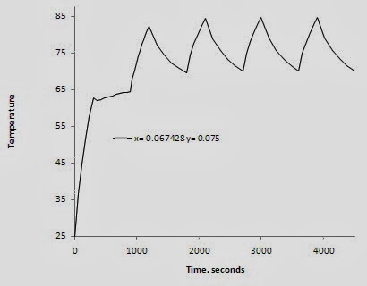
A typical natural convection heat sink is used. It is 93.65 mm wide and 75 mm long with a base plate thickness of 6.35 mm, fin spacing of 10.14 mm, fin thickness of 1.5 mm and fin height of 24.5 mm - see the attached.  Two heat sources are used, 9 and 18 W located and sized as shown.  The heat load duty cycle is 5 minutes at full power followed by 10 minutes at 1/2 power.  The heat sink is assumed to be oriented with the fin channels vertical in free air at 25 C.

The maximum predicted heat sink temperature is 87.7 C for a corresponding delta T = 62.7 C.  The time/temperature plot is shown below for the maximum temperature location.

Time/Temperature Plot.

After ~ 4 full power cycles the temperature has peaked.  This animation shows the heat sink temperatures over the heat cycles.

Animation of the HX Temperatures over Time.

If the full power heat load is conservatively used then the steady state maximum predicted temperature is 98.9 C or a delta  T = 73.9 C.  This is a ~ 18% increase over the transient solution. 

Steady Temperatures Assuming Continuous Full Power.

If the cyclic heat load was predictably constant then the heat sink could conceivably be reduced in size for space and expense savings.

The above analysis was done using the Heat Sink module of the XL4Sim series.  The full analysis was setup and completed in less than 2 hours demonstrating the ease of use and efficiency of the simulation tool.

Comments welcome.