This blog shows how MS Excel and Google Sheets can be used for engineering and other technical applications. Examples of their use will be given and discussed. They will be in the form of COM Add-ins, macros, templates, user functions, Google scripts, simple forms, online calculators and other.
Discussion ideas are welcome.
Many thermal management systems have unsteady heat loads. Heat sink design and/or selection can be considered with these unsteady loads in mind.
An example of a natural convection finned heat sink is used to show how the thermal mass of the heat sink can be used to reduce its required cooling capacity. Generally the effects of thermal mass are intuitive but calculating the benefits can sometimes be challenging. This example shows an easy and quick simulation for evaluating the potential benefits of the transient behavior.
XL4Sim Simulation of a Transient, Naturally Cooled Heat Sink.
A typical natural convection heat sink is used. It is 93.65 mm wide and 75 mm long with a base plate thickness of 6.35 mm, fin spacing of 10.14 mm, fin thickness of 1.5 mm and fin height of 24.5 mm - see the attached. Two heat sources are used, 9 and 18 W located and sized as shown. The heat load duty cycle is 5 minutes at full power followed by 10 minutes at 1/2 power. The heat sink is assumed to be oriented with the fin channels vertical in free air at 25 C.
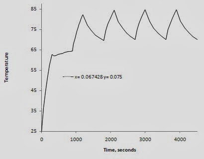
The maximum predicted heat sink temperature is 87.7 C for a corresponding delta T = 62.7 C. The time/temperature plot is shown below for the maximum temperature location.
Time/Temperature Plot.
After ~ 4 full power cycles the temperature has peaked. This animation shows the heat sink temperatures over the heat cycles.
Animation of the HX Temperatures over Time.
If the full power heat load is conservatively used then the steady state maximum predicted temperature is 98.9 C or a delta T = 73.9 C. This is a ~ 18% increase over the transient solution.
Steady Temperatures Assuming Continuous Full Power.
If the cyclic heat load was predictably constant then the heat sink could conceivably be reduced in size for space and expense savings.
The above analysis was done using the Heat Sink module of the XL4Sim series. The full analysis was setup and completed in less than 2 hours demonstrating the ease of use and efficiency of the simulation tool.
Attached is an MS Excel Macro of a 2 degree-of-freedom vibration simulation model that calculates the response to a random vibration input - PSD (power spectral density).
2-DOF Random Vibration Dashboard.
Vibration isolation strategy for tonal systems is generally straight forward where one can isolate by using soft isolators that put the forcing frequencies above the isolation frequency. Or tune between forcing frequencies. Sway space, damping, isolator fatigue and other considerations are needed as well.
For random vibration input the strategy is not so straight forward. In theory, all frequencies between the limits of the PSD are present. Any system natural frequency within this range would be set into resonance. Sway space, damping and other considerations are still important.
Typical PSD Curve.
The simulation model of the macro uses 2 masses with the random vibration input at the base. It could simulate the frame of a car that has an electrical containment box attached to it that in turn has a circuit board mounted inside the box. The circuit board is depicted as body (mass) 2, the box depicted as body (mass) 1 and the car body the rigid body that randomly vibrates the box from road irregularities, drive-train, and other sources..
2 DOF Vibration Model.
The simulation model has the following features:
M1, M2, K01 and K12 are input by the user.
Modal damping ratio can be input.
A PSD curve can be input.
A user defined gravitational constant is input.
Any consistent set of dimensional units can be used.
The simulation can calculate:
PSD Grms value; the 2 natural frequencies and mode shapes.
Mode shapes can be animated.
RMS response G's and relative displacement values.
A pseudo time series can be determined from the PSD.
A dynamic transient analysis of the time series can be done and response values determined.
The transient response can be animated.
Random Vibration Response.
For a typical example the following was simulated: a 5 lb circuit board mounted inside a 50 lb box which is mounted to a car frame that has a uniform 5-500 Hz 0.5 G2/Hz random vibration input. Low modal damping of 2% was also assumed. Two scenarios were evaluated.
First, it was assumed the circuit board was on mounts and/or isolators that gave it a natural frequency of 25 Hz. The box was then mounted to the car frame by a progressively softer attachment. Starting virtually hard mounted and then softened to a a frequency near the 25 Hz. The results are shown below. The box acceleration response is initially high because it's primary mode (box-to-car frame mode) is within the 500 Hz PSD range. As its mounting gets softer that mode drops in frequency and the response drops. As that frequency gets closer to the circuit board mode frequency they start to dynamically couple and more response is felt by the circuit board. As the frequency ratio (2nd mode-to-1st mode) approaches 2 from the right side of the chart the circuit response starts to increase dramatically.
Body 2 at 25 Hz and Body 1 Mounted with Varying Stiffnesses.
The second scenario was to assume the box-to-car frame natural frequency is 25 Hz and the circuit board mounted progressively softer from starting with a "hard" mount case. The results are below.
The trends are similar to the first scenario except that the box response starts out relatively low because it's already at a low natural frequency and the circuit board is isolated by the box from the car. As the circuit board mounting becomes softer the acceleration response of both the box and circuit board increase. At a frequency ratio of 2 they are feeling large responses from their mode coupling. In this case the mode 2 is predominately the circuit board mode. Whereas in the first scenario the box was predominately mode 2.
The take ways from this simple study are: 1) For 2 DOF system keeping the 2 modes separated by a frequency ratio of at least 2 (an octave) or more would be desirable from an acceleration response prospective. A frequency ratio greater than 4 appears to offer diminishing returns. 2) Isolating the box is preferred over isolating the circuit board assuming no other considerations make this undesirable like available sway space for the box which increases as the isolation frequency drops.
The attached spreadsheet summarizes the details shown in the two preceding charts.
Of course, other factors need to be evaluated. For example, this simple case used a uniform PSD input. Most PSD's decrease at the higher frequencies. Additional damping can be used, especially if elastomer isolators are used.
Note: The MS Excel Macro has been code signed with an independent code signing certificate to allow higher security settings. The macro has a time limit of 1/1/2015. Updated versions will be accessible at www.XL4Sim.com.
This is a link to an Excel COM Add-in for a module that was written to do beam analyses. It will do statics, modal, steady response and transient response on beams with varying materials and section properties. Loads include concentrated forces and weights, linearly distributed and beam weight. Boundaries include free, simply-supported, fixed, deflection, slope, translational spring and rotational spring.
The Add-in can be used in any version of Excel from 97-2003 and later and will create the menu structure for the appropriate version. Examples cases are provided to show how to use and setup models.
Note:The Add-in can be turned off within Excel or deleted by the "removing programs" option in Windows.
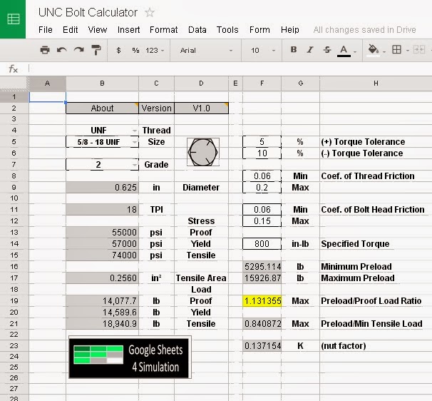
This link is the Excel 2007 version of the Calculator. This is a macro and has been trusted source code signed with a third party (Thawte) certificate so it doesn't jam up your Excel security settings if you want to download it.
It includes SAE 429 UNC and UNF bolts and ISO Metric bolts with all the common tensile strength grades. The bolt type (in-lb or metric), thread type (fine or coarse), size and grade are selected by dropdown lists. The preload calculation uses a user input range of torque tolerance, thread friction range and bolt head friction range. The maximum and minimum preloads are determined and compared to the proof and tensile loads for the selected grade. For reference the "nut factor", K is also calculated and given.
This link is a Google sheets version of the SAE 429 Bolt Preload Calculator for the shared "view only" version. For an editable and shared version use this link. Any changes will automatically be added to the shared version. I would suggest making a copy of the original shared version and use and control that as you wish.
(Disclaimer: I've just starting using Google sheets and am still learning how the Google "My Drive" and sharing system works. This is my current understanding and seems to work with the testing I've done. The Google scripting I've used to do the sheet calculations and load the drop-downs on the active sheet works fine and should work for the editable version. By design the "view only" shared version of the sheet will be completely inactive.)
The Google sheets version currently only includes the SAE 429 UNC and UNF bolts with the common grades. As mentioned Google script is used to populate the drop down lists and run the calculations.
Multiple scenarios can be evaluated and saved by copying the workbook and/or worksheet. The macro and script get copied along with the worksheet which can be named anything. All normal spreadsheet functionality is maintained.
The attached spreadsheet is an example of using the Excel Solver function to estimate parameters for the nonlinear transient thermal model of a battery used on a hybrid vehicle.
The temperature data was collected on a rack of batteries that were repeatedly charged and discharged. The batteries were cooled by natural convection. The data used in the example analysis was collected over roughly a 24 hour period. The ambient temperature at the rack ranged from ~ 32.5 to 37.5 C.
The temperature trace used was from a thermocouple located on the case of one of the batteries.
The first pass model was a single lumped mass of an individual battery with natural convection cooling and joule heating. This was represented by:
McpdT/dt = Q - hA(T-Ta) where Mcp is the thermal mass, Q the heat load, hA the heat transfer coefficient times the surface area, and Ta the ambient temperature.
The heat load, Q, was defined by QfI2 = Qcharge I2 for the charge cycle and QdischargeI2. The electrical current is I and ranges from 240 amps for the charge and 300 amps for the discharge. Note: For this example it is assumed that any heating from chemical kinetics is secondary and captured by the Q terms.
The natural convection, hA, is defined by Ch(T-Ta)x(T-Ta). This is based on natural convection heat transfer coefficients being estimated by CRan where Ra is the Rayleigh number and the exponent n ranging from .25 to .35 depending on the surface type.
The overall equation looks like
McpdT/dt = QfI2 - Ch(T-Ta)1+x.
This can be setup in a finite difference form in time as
The spreadsheet is setup with this form of the model.
Solver can now be used to find the best fit values for Qf, Ch, cp, Ch and x. Solver will find local minima so several starting values should tried. The constraints can also be used if reasonable values are known. For example, the convective heat transfer coefficient, x, should be somewhere between . 2 and .35 based on textbook values for flat surfaces with natural convection. Reference: "Fundamentals of Heat and Mass Transfer" 4th Edition by Incropera and DeWitt pgs 492 - 501.
The values could be determined by using the full time period, however, more accuracy can be gained by breaking the regression into sections. For example, the cool-down section can be used with the Qf term set to 0.0 to find fits for Ch, x and cp. The heat-up section can then be used to find Qf charge and discharge using the previously determined Ch and x values. The cp value can either be used from the cool-down or see what value fits the heat-up.
The full model can then be checked with the best fit values from each of the sections. Some refinement is necessary to better fit the overall time period and this was done manually.
Each of the worksheets used for this approach is given in the attached workbook.